• 写在前面
• 问题描述
  • RBF
    • 1. Logarithmic
    • 2. Inverse-type
    • 3. Reciprocal
  • ZBF
  • 两者的联系
• CBF构建
  • RCBF
  • ZCBF
• QP设计
  • ES-CLF
  • CLF-CBF QP

写在前面

原论文：Control Barrier Function Based Quadratic Programs for Safety Critical Systems.

本文为近期阅读的论文(Ames 2017)^[1]的笔记。该论文介绍了两种barrier function，即reciprocal barrier function (RBF)和zeroing barrier function (ZBF)，目的是将它们扩展为control barrier function (CBF)，并以二次规划(QP)形式与control Lyapunov function (CLF)结合起来，实现带有约束的控制器。

针对给定集合$\mathcal C$，如果$B(x)$在集合边界处无界，即$B(x)\to \infty$ as $x\to\partial \mathcal C$，则称函数$B$为RBF；如果$h(x)$在集合边界处为0，即$h(x)\to 0$ as $x\to\partial \mathcal C$，则称函数$h$为ZBF。以上任意一种情况的$B$或$h$满足Lyapunov-like条件，则可以保证$\partial \mathcal C$的不变性(forward invariance)。

问题描述

考虑非线性系统

$\dot x=f(x)\qquad(1)$

其中$x\in\mathbb R^n$，假设$f$是locally Lipschitz。集合$\mathcal C$对于(1)不变(forward invariant)，如果对每一个$x_0\in\mathcal C$，都有$x(t)\in\mathcal C$，$\forall t\in[0,\infty)$。

RBF

问题1：给定闭集$\mathcal C:=\{x\in\mathbb R^n|h(x)\geq 0 \}$，确定函数$B:\operatorname{int}(\mathcal C)\to \mathbb R$并构建CBF使得$\operatorname{int}(\mathcal C)$不变，其中$h:\mathbb R^n\to\mathbb R$是连续可微函数。同时假设$\mathcal C$非空没有孤立点(isolated point)，即$\operatorname{int}(\mathcal C)\neq \emptyset$，$\overline{\operatorname{int}(\mathcal C)}=\mathcal C$。

1. Logarithmic

选取logarithmic barrier function candidate

$B(x)=-\log\left(\frac{h(x)}{1+h(x)} \right)\qquad (2)$

满足$\inf_{x\in\operatorname{int}(\mathcal C)}B(x)\geq 0$，$\lim_{x\to\partial\mathcal C}B(x)=\infty$。

设计条件

$\dot B\leq \frac{\gamma}{B}，\qquad (3)$

使得$B$在远离边界时可以增大，越接近边界增大速率越接近于0。

证明：对(2)求导代入条件中，得到$\dot h\geq \frac{\gamma(h+h^2)}{\log(\frac{h}{1+h})}$，由比较引理(Comparison Lemma)得到，如果$x_0\in\operatorname{int}(\mathcal C)$，那么$\forall t\geq 0$，有

$h(x(t,x_0))\geq \frac{1}{\exp\left(\sqrt{2\gamma t+\log^2\left(\frac{h(x_0)+1}{h(x_0)}\right)}\right)-1}>0$

成立，即$x(t,x_0)\in\operatorname{int}(\mathcal C)$，$\forall t\geq 0$。该函数下界收敛于0。

2. Inverse-type

选取inverse-type barrier candidate

$B(x)=\frac{1}{h(x)}。$

同理，有$h(x(t,x_0))\geq \frac{1}{\sqrt{2\gamma t+\frac{1}{h^2(x_0)}}}>0$。该函数下界始终大于0。

3. Reciprocal

定义1：对动态系统(1)，一个连续可微函数$B: \operatorname{int}(\mathcal C)\to \mathbb R$是集合$\mathcal C$的RBF，如果存在$\mathcal K$类函数$\alpha_1$、$\alpha_2$、$\alpha_3$使得，$\forall x\in\operatorname{int}(\mathcal C)$，

$\begin{aligned} \frac{1}{\alpha_1(h(x))}\leq B(x)&\leq \frac{1}{\alpha_2(h(x))}，\\ L_f B(x)&\leq \alpha_3(h(x))。 \end{aligned}$

定理1：给定动态系统(1)和由连续可微函数$h$定义的集合$\mathcal C$，如果存在$B$是一个RBF，那么$\operatorname{int}(\mathcal C)$对于(1)是不变的。

ZBF

定义2：对于$a,b>0$，连续函数$\alpha:(-b,a)\to (-\infty,\infty)$被认为属于扩展$\mathcal K$类函数，如果它严格单调增且$\alpha(0)=0$。

扩展$\mathcal K$类函数和$\mathcal K$类函数区别在于，定义域和值域可以取负数，如果令$b=0$，值域为$[0,\infty)$，那么扩展$\mathcal K$类函数即$\mathcal K$类函数。

定义3：对动态系统(1)，一个连续可微函数$h:\mathbb R^n\to \mathbb R$是集合$\mathcal C$的ZBF，如果存在扩展$\mathcal K$类函数$\alpha$和集合$\mathcal D$($\mathcal C\subseteq \mathcal D\subset \mathbb R^n$)使得，$\forall x\in\mathcal D$，

$L_fh(x)\geq -\alpha(h(x))。$

注意：将$h$定义在一个比$\mathcal C$大的集合$\mathcal D$上可以考虑模型扰动的影响。

命题1：给定动态系统(1)和由连续可微函数$h$定义的集合$\mathcal C$，如果$h$是一个定义在$\mathcal D$上的ZBF，那么$\operatorname{int}(\mathcal C)$对于(1)是不变的。

证明：对任意$x\in\partial \mathcal C$，$\dot h(x)\geq -\alpha(h(x))=0$。由Nagumo定理知，集合$\mathcal C$是不变的。

Nagumo定理^[2]：考虑系统$\dot x=f(x)$，假设对每个集合$\mathcal D$中的初始值，系统都有一个全局唯一解。令$\mathcal C\subseteq \mathcal D$是闭凸集。那么集合$\mathcal C$对系统是不变的，当且仅当$f(x)\in T_{\mathcal C}(x)$(切锥)，$\forall x\in\mathcal C$。

因为当$x\in\operatorname{int} \mathcal C$，$T_{\mathcal C}=\mathbb R^n$，所以只用关心$x\in\partial \mathcal C$的情况。由于$h(x)$处处光滑，故切锥为半平面。当$x\in\partial \mathcal C$，$L_fh(x)=\nabla h^T(x)f(x)\geq 0$，即$f(x)$和梯度夹角小于$\frac{\pi}{2}$，所以$f(x)\in T_{\mathcal C}(x)$，如下图所示。

Nagumo定理对非凸集合也成立，但是唯一解要求必须满足。

命题2：令$h:\mathcal D\to \mathbb R$为定义在开集$\mathcal D\subseteq \mathbb R^n$上的连续可微函数。如果$h$是系统(1)的ZBF，那么由$h$定义的集合$\mathcal C$渐进稳定。

命题2告诉我们，即使初始位置在集合$\mathcal C$之外，也有$x$渐进收敛于$\mathcal C$。

两者的联系

命题3：给定动态系统(1)和由连续可微函数$h$定义的集合$\mathcal C$。如果$\mathcal C$是不变的，那么$h|_{\mathcal C}$是$\mathcal C$上定义的ZBF。

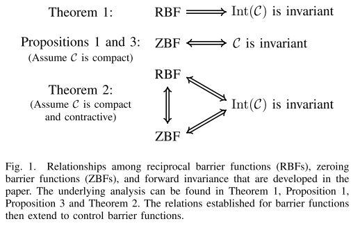
命题1和3共同证明，集合$\mathcal C$是不变的，当且仅当存在一个ZBF。同样的对RBF，也能证明必要性，见原论文的定理2，这里不再详述。

RBF、ZBF和集合不变性的联系如下图所示。

CBF构建

类似于利用Lyapunov函数构建CLF的方法，我们也可以利用RBF和ZBF构建CBF。

RCBF

考虑仿射控制系统

$\dot x=f(x)+g(x)u，\qquad (4)$

其中$f$和$g$局部Lipschitz，$x\in\mathbb R^n$，$u\in U\subset\mathbb R^m$。

定义4：对系统(4)和由连续可微函数$h$定义的集合$\mathcal C$，一个连续可微函数$B: \operatorname{int}(\mathcal C)\to \mathbb R$是RCBF，如果存在$\mathcal K$类函数$\alpha_1$、$\alpha_2$、$\alpha_3$使得，$\forall x\in\operatorname{int}(\mathcal C)$，

$\begin{aligned} \frac{1}{\alpha_1(h(x))}\leq B(x)&\leq \frac{1}{\alpha_2(h(x))}，\\ \inf_{u\in U}[L_f B(x)+L_g B(x)u&-\alpha_3(h(x))]\leq0 。 \end{aligned}$

RCBF $B$局部Lipschitz连续，如果$\alpha_3$和$\frac{\partial B}{\partial x}$都局部Lipschitz连续。

给定RCBF $B$，$\forall x\in \operatorname{int}(\mathcal C)$，定义集合

$K_{\operatorname{rcbf}}(x)=\{u\in U|L_fB(x)+L_g B(x)u-\alpha_3(h(x))\leq 0 \}。$

推论1：考虑集合$\mathcal C$，令$B$是系统(4)的RCBF。那么任意局部Lipschitz连续的控制器$u:\operatorname{int}(\mathcal C)\to U$使得$u(x)\in K_{\operatorname{rcbf}}(x)$都能保证集合$\operatorname{int}(\mathcal C)$的不变性。

ZCBF

定义5：对系统(4)和由连续可微函数$h:\mathbb R^n\to \mathbb R$定义的集合$\mathcal C$，$h$是定义在集合$\mathcal D$上($\mathcal C\subseteq \mathcal D\subset \mathbb R^n$)的ZCBF，如果存在扩展$\mathcal K$类函数$\alpha$使得，

$\sup_{u\in U}[L_f h(x)+L_g h(x)u+\alpha(h(x))]\geq 0 。$

ZCBF $h$局部Lipschitz连续，如果$\alpha$和$\frac{\partial h}{\partial x}$都局部Lipschitz连续。

给定ZCBF $h$，$\forall x\in \mathcal D$，定义集合

$K_{\operatorname{zcbf}}(x)=\{u\in U|L_f h(x)+L_g h(x)u+\alpha(h(x))\geq 0 \}。$

推论2：考虑集合$\mathcal C$，令$h$是集合$\mathcal D$上的ZCBF。那么任意局部Lipschitz连续的控制器$u:\mathcal D\to U$使得$u(x)\in K_{\operatorname{zcbf}}(x)$都能保证集合$\mathcal C$的不变性。

QP设计

用QP来协调控制效果和安全约束。考虑仿射控制系统

$\begin{bmatrix} \dot x_1\\ \dot x_2 \end{bmatrix}=\begin{bmatrix} f_1(x_1,x_2)\\ f_2(x_1,x_2) \end{bmatrix}+\begin{bmatrix} g_1(x_1,x_2)\\ 0 \end{bmatrix}u。$

其中$x_1\in X$是可控状态(或输出)，$x_2\in Z$是不可控状态。

ES-CLF

定义6：连续可微函数$V:X\times Z\to \mathbb R$是ES-CLF(exponetial stabilizing control Lyapunov function)，如果存在正常数$c_1,c_2,c_3> 0$使得$\forall x=(x_1,x_2)\in X\times Z$，下列不等式成立，

$c_1\|x_1\|^2\leq V(x)\leq c_2\|x_1\|^2，\\ \operatorname{inf}_{u\in U}[L_f V(x)+L_g V(x)u+c_3V(x)]\leq 0。$

定义集合

$K_{\operatorname{clf}}(x)=\{u\in U|L_f V(x)+L_g V(x)u+c_3 V(x)\leq 0 \}。$

局部Lipschitz控制器$u:X\times Z\to U$满足

$u(x)\in K_{\operatorname{clf}}(x) \Rightarrow \|x_1(t)\|\leq \sqrt{\frac{c_2}{c_1}}e^{-\frac{c_3}{2}t}\|x_1(0)\|。$

CLF-CBF QP

对于RCBF，考虑如下形式的QP问题

$\begin{aligned} \boldsymbol u^*(x)&= {\arg\min}_{\boldsymbol{u}=(u,\delta)\in\mathbb R^m\times \mathbb R} \frac{1}{2}\boldsymbol u^TH(x)\boldsymbol u+F(x)^T\boldsymbol u\\ \operatorname{s.t.} &\quad \begin{aligned}L_fV(x)+L_gV(x)u+c_3 V(x)-\delta&\leq 0\\ L_f B(x)+L_g B(x)u-\alpha(h(x))&\leq 0 \end{aligned} \end{aligned}$

其中，$c_3>0$是常数，$\alpha$是$\mathcal K$类函数，$H(x)\in \mathbb R^{(m+1)\times(m+1)}$正定，$F(x)\in\mathbb R^{m+1}$。

下述定理提供$\boldsymbol u^*(x)$局部Lipschitz连续的充分条件，保证控制器的局部存在性和解的唯一性这些前提条件，从而推论1、2得以应用。

定理3：假设$f,g,B,V,H,F$都局部Lipschitz连续。再假设相对度为1，即$L_g B(x)\neq 0$，$\forall x\in\operatorname{int}(\mathcal C)$。那么CLF-CBF QP的解$\boldsymbol u^*(x)$在$\operatorname{int}(\mathcal C)$上局部Lipschitz连续。另外，$\boldsymbol u^*(x)$可以写成一个闭环解析式。

证明：令$\boldsymbol v=\boldsymbol u+H^{-1}F$，$\langle \boldsymbol v,\boldsymbol v\rangle=\boldsymbol v^TH\boldsymbol v$，

$A =[a_1,a_2]= \begin{bmatrix} L_g V&L_g B\\ -1&0 \end{bmatrix}，b=\begin{bmatrix} -L_f V-c_3 V\\ -L_f B+\alpha(h) \end{bmatrix}+A^TH^{-1}F。$

原QP问题重写为

$\begin{aligned} \boldsymbol v^*=&\arg\min \frac{1}{2}\langle \boldsymbol v,\boldsymbol v \rangle\\ \operatorname{s.t.}&\quad A^T\boldsymbol v\leq b \end{aligned}$

因为代价函数是凸的且不等式为线性，所以KKT条件是充要条件。令$G=A^TH^{-1}A=\begin{bmatrix}a_1^TH^{-1}a_1&a_1^TH^{-1}a_2\\ a_2^TH^{-1}a_1& a_2^TH^{-1}a_2\end{bmatrix}$是Gram矩阵，由于$a_1$、$a_2$线性无关，$G$是正定的。由KKT条件可知，该问题的唯一解是$\boldsymbol v^*=H^{-1}A\lambda$，其中$\lambda\in\mathbb R^2$，且满足

$\left\{ \begin{aligned} 0&\geq\lambda，\\ 0&\geq A^TH^{-1}A\lambda-b=G\lambda-b，\\ 0&=\lambda^T(A^TH^{-1}A\lambda-b)=\lambda^T(G\lambda-b)。 \end{aligned} \right.$

可知，若$[G\lambda-b]_i<0$，则$\lambda_i=0$。($G\lambda-b$和$\lambda$不可能同时小于0，相互垂直的向量肯定在不同象限或者坐标轴。) 又因为$G$正定，$G_{11}>0$，且$G_{11}G_{22}-G_{12}G_{21}>0$。由schur complement condition，$G_{22}>0$。

分类讨论：

• $[G\lambda-b]_1<0$，$[G\lambda-b]_2=0$

• $[G\lambda-b]_1=0$，$[G\lambda-b]_2<0$

• $[G\lambda-b]_1<0$，$[G\lambda-b]_2<0$

• $[G\lambda-b]_1=0$，$[G\lambda-b]_2=0$

情况1：将$\lambda_1=0$代入$[G\lambda-b]_2=0$，解出$\lambda_2=b_2/G_{22}\leq 0$。再将$\lambda_1=0$代入$[G\lambda-b]_1=0$，得到$G_{12}b_2-G_{22}b_1<0$。即，当$G_{12}b_2-G_{22}b_1<0$，$b_2\leq 0$时，$\lambda=\begin{bmatrix}0\\b_2/G_{22} \end{bmatrix}$；

情况2：将$\lambda_2=0$代入$[G\lambda-b]_1=0$，解出$\lambda_1=b_1/G_{11}\leq 0$。再将$\lambda_2=0$代入$[G\lambda-b]_2=0$，得到$G_{21}b_1-G_{11}b_2<0$。即，当$G_{21}b_1-G_{11}b_2<0$，$b_1\leq 0$时，$\lambda=\begin{bmatrix}b_1/G_{11}\\ 0 \end{bmatrix}$；

情况3：当$b_1,b_2>0$时，$\lambda=[0,0]^T$；

情况4：此时$\lambda=G^{-1}b\leq 0$。

综上所述，对$x\in\operatorname{int}(\mathcal C)$，$\lambda$可写为如下闭环解析形式：

当$G_{12}\min\{b_2,0\}-G_{22}b_1<0$时，$\lambda=\begin{bmatrix}0\\\min\{b_2,0\}/G_{22} \end{bmatrix}$；当$G_{21}\min\{b_1,0\}-G_{11}b_2<0$时，$\lambda=\begin{bmatrix}\min\{b_1,0\}/G_{11}\\ 0 \end{bmatrix}$；其他情况时，$\lambda=\begin{bmatrix}\min\{G_{22}b_1-G_{21} b_2\}\\ \min\{G_{11}b_2-G_{12}b_1 \}\end{bmatrix}/(G_{11}G_{22}-G_{12}G_{21})$。(最后一个情况$\lambda$不可能为0，因为$G$的行向量线性无关。)

对于ZCBF，考虑如下形式的QP问题

$\begin{aligned} \boldsymbol u^*(x)&= {\arg\min}_{\boldsymbol{u}=(u,\delta)\in\mathbb R^m\times \mathbb R} \frac{1}{2}\boldsymbol u^TH(x)\boldsymbol u+F^T(x)\boldsymbol u\\ \operatorname{s.t.} &\quad \begin{aligned}L_fV(x)+L_gV(x)u+c_3 V(x)-\delta&\leq 0\\ -L_f h(x)-L_g h(x)u-\alpha(h(x))&\leq 0 \end{aligned} \end{aligned}$

其中，$c_3>0$是常数，$\alpha$是$\mathcal K$类函数，$H(x)\in \mathbb R^{(m+1)\times(m+1)}$正定，$F(x)\in\mathbb R^{m+1}$。同理，我们有关于ZCBF的定理。

定理4：假设$f,g,h,V,H,F$都局部Lipschitz连续。再假设相对度为1，即$L_g h(x)\neq 0$，$\forall x\in\mathcal D$。那么CLF-CBF QP的解$\boldsymbol u^*(x)$在$\mathcal D$上局部Lipschitz连续，且解可以写成一个闭环解析式。

---

1. Ames, A. D., Xu, X., Grizzle, J. W., & Tabuada, P. (2017). Control Barrier Function Based Quadratic Programs for Safety Critical Systems. IEEE Transactions on Automatic Control, 62(8), 3861–3876. https://doi.org/10.1109/TAC.2016.2638961 ↩︎

2. Blanchini, F. (1999). Set invariance in control. Automatica. Elsevier Science Ltd. https://doi.org/10.1016/S0005-1098(99)00113-2 ↩︎